Autoencoders for Representation Learning

import os
import shutil

base = "/kaggle/working/FashionMNIST/raw"
os.makedirs(base, exist_ok=True)

src = "/kaggle/input/datasets/organizations/zalando-research/fashionmnist"

files = [
    "train-images-idx3-ubyte",
    "train-labels-idx1-ubyte",
    "t10k-images-idx3-ubyte",
    "t10k-labels-idx1-ubyte"
]

for f in files:
    shutil.copy(
        os.path.join(src, f),
        os.path.join(base, f)
    )

print("Files copied successfully")

from torchvision import datasets, transforms
from torch.utils.data import DataLoader

transform = transforms.ToTensor()

train_data = datasets.FashionMNIST(
    root="/kaggle/working",
    train=True,
    download=False,
    transform=transform
)

test_data = datasets.FashionMNIST(
    root="/kaggle/working",
    train=False,
    download=False,
    transform=transform
)

train_loader = DataLoader(train_data, batch_size=128, shuffle=True)
test_loader = DataLoader(test_data, batch_size=128, shuffle=False)

print("Dataset loaded successfully!")
print(f"Training samples: {len(train_data)} | Test samples: {len(test_data)}")

# Define class names for FashionMNIST
classes = [
    'T-shirt/top', 'Trouser', 'Pullover', 'Dress', 'Coat',
    'Sandal', 'Shirt', 'Sneaker', 'Bag', 'Ankle boot'
]

def display_one_from_each_class(dataset):
    found_classes = {}
    idx = 0
    
    # Loop until we find one of each (0-9)
    import os
    import shutil
    base = "/kaggle/working/FashionMNIST/raw" 
    os.makedirs(base, exist_ok=True)
    src = "/kaggle/input/fashionmnist"
    files = [
        "train-images-idx3-ubyte", "train-labels-idx1-ubyte", 
        "t10k-images-idx3-ubyte", "t10k-labels-idx1-ubyte"
    ]
    for f in files:
        shutil.copy(os.path.join(src, f), os.path.join(base, f))
    print("Files copied successfully")
    
    while len(found_classes) < 10: 
        img, label = dataset[idx]
        if label not in found_classes: 
            found_classes[label] = img
        idx += 1
        
    # Plotting
    plt.figure(figsize=(15, 5))
    for label, img in sorted(found_classes.items()): 
        plt.subplot(2, 5, label + 1)
        # Convert tensor to numpy and remove channel dim for grayscale
        plt.imshow(img.squeeze(), cmap='gray') 
        plt.title(classes[label])
        plt.axis('off')
    plt.tight_layout() 
    plt.show()

# Execute the function
display_one_from_each_class(train_data)

# Architecture: Deeper network with BatchNorm, Dropout, and 2D latent space
# Progression: 784 → 512 → 256 → 128 → 64 → 32 → 16 → 8 → 4 → 2
class Autoencoder(nn.Module):
    def __init__(self):
        super().__init__()
        
        # Deeper encoder: Compressing from 784 down to 2
        self.encoder = nn.Sequential(
            nn.Flatten(),
            nn.Linear(784, 512),
            nn.BatchNorm1d(512),
            nn.ReLU(),
            nn.Dropout(0.1),
            
            nn.Linear(512, 256),
            nn.BatchNorm1d(256),
            nn.ReLU(),
            
            nn.Linear(256, 128),
            nn.BatchNorm1d(128),
            nn.ReLU(),
            
            nn.Linear(128, 64),
            nn.BatchNorm1d(64),
            nn.ReLU(),
            
            nn.Linear(64, 32),
            nn.BatchNorm1d(32),
            nn.ReLU(),
            
            nn.Linear(32, 16),
            nn.BatchNorm1d(16),
            nn.ReLU(),
            
            nn.Linear(16, 8),
            nn.BatchNorm1d(8),
            nn.ReLU(),
            
            nn.Linear(8, 4),
            nn.BatchNorm1d(4),
            nn.ReLU(),
            
            nn.Linear(4, 2)  # Latent space (2D for visualization)
        )
        
        # Deeper decoder: Reconstructing from 2 back to 784
        self.decoder = nn.Sequential(
            nn.Linear(2, 4),
            nn.BatchNorm1d(4),
            nn.ReLU(),
            
            nn.Linear(4, 8),
            nn.BatchNorm1d(8),
            nn.ReLU(),
            
            nn.Linear(8, 16),
            nn.BatchNorm1d(16),
            nn.ReLU(),
            
            nn.Linear(16, 32),
            nn.BatchNorm1d(32),
            nn.ReLU(),
            
            nn.Linear(32, 64),
            nn.BatchNorm1d(64),
            nn.ReLU(),
            
            nn.Linear(64, 128),
            nn.BatchNorm1d(128),
            nn.ReLU(),
            
            nn.Linear(128, 256),
            nn.BatchNorm1d(256),
            nn.ReLU(),
            
            nn.Linear(256, 512),
            nn.BatchNorm1d(512),
            nn.ReLU(),
            
            nn.Linear(512, 784),
            nn.Sigmoid()  # Use Sigmoid for pixel values between [0, 1]
        )
    
    def forward(self, x):
        z = self.encoder(x)
        out = self.decoder(z)
        # Reshape output back to image dimensions if necessary for your loss function
        # out = out.view(-1, 1, 28, 28)
        return out, z

print("Model architecture defined successfully!")

# BASIC AUTOENCODER TRAINING
# Trains on clean images only — no noise added (clean → clean)

device = torch.device("cuda" if torch.cuda.is_available() else "cpu")
basic_model = Autoencoder().to(device)

criterion_mse = nn.MSELoss()
criterion_l1 = nn.L1Loss()
optimizer_basic = optim.Adam(basic_model.parameters(), lr=0.001)
scheduler_basic = optim.lr_scheduler.ReduceLROnPlateau(optimizer_basic, mode='min', patience=5)

epochs = 100
best_loss_basic = float('inf')

for epoch in range(epochs):
    basic_model.train()
    total_loss = 0

    for images, _ in train_loader:
        images = images.to(device)
        outputs, _ = basic_model(images)

        loss_mse = criterion_mse(outputs, images.view(images.size(0), -1))
        loss_l1 = criterion_l1(outputs, images.view(images.size(0), -1))
        loss = 0.7 * loss_mse + 0.3 * loss_l1

        optimizer_basic.zero_grad()
        loss.backward()
        torch.nn.utils.clip_grad_norm_(basic_model.parameters(), max_norm=1.0)
        optimizer_basic.step()
        total_loss += loss.item()

    avg_loss = total_loss / len(train_loader)
    scheduler_basic.step(avg_loss)

    if avg_loss < best_loss_basic:
        best_loss_basic = avg_loss

    if (epoch + 1) % 5 == 0:
        print(f"Epoch [{epoch+1}/{epochs}] Loss: {avg_loss:.4f}")

print(f"\nTraining completed! Best Loss: {best_loss_basic:.4f}")

# VISUALIZATION: BASIC RECONSTRUCTION
# Display original and reconstructed images side-by-side (no noise — clean input only)

basic_model.eval()
images, _ = next(iter(test_loader))
images = images.to(device)

with torch.no_grad():
    reconstructed_basic, _ = basic_model(images)

# Display 8 samples
n = 8
plt.figure(figsize=(12, 4))

for i in range(n):
    # Original
    plt.subplot(2, n, i+1)
    plt.imshow(images[i].cpu().squeeze(), cmap='gray')
    plt.axis('off')

    # Reconstructed
    plt.subplot(2, n, i+1+n)
    plt.imshow(reconstructed_basic[i].view(28,28).cpu(), cmap='gray')
    plt.axis('off')

plt.tight_layout()
plt.show()

print("Basic reconstruction visualization completed!")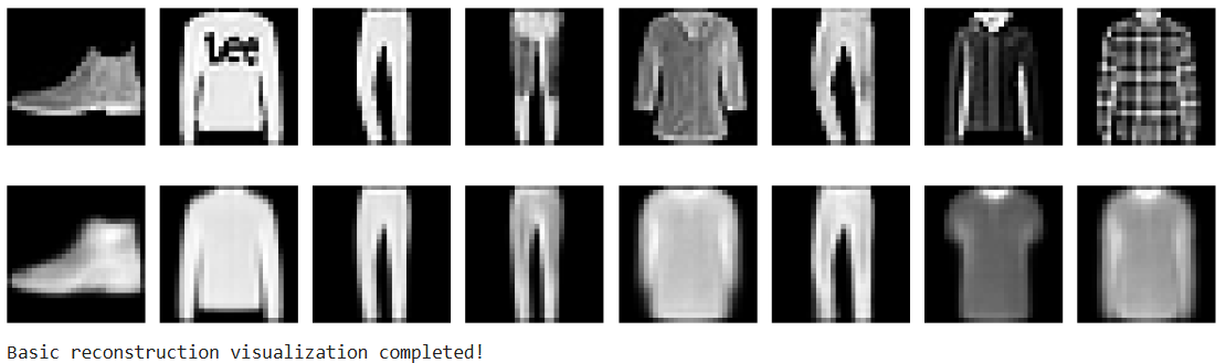

# DENOISING AUTOENCODER TRAINING
# Uses combined MSE + L1 loss with gradient clipping
# Trains on noisy images, reconstructs clean ones (noisy → clean)

def add_noise(x, noise_factor=0.25):
    noisy = x + noise_factor * torch.randn_like(x)
    return torch.clamp(noisy, 0., 1.)

device = torch.device("cuda" if torch.cuda.is_available() else "cpu")
model = Autoencoder().to(device)

criterion_mse = nn.MSELoss()
criterion_l1 = nn.L1Loss()
optimizer = optim.Adam(model.parameters(), lr=0.001)
scheduler = optim.lr_scheduler.ReduceLROnPlateau(optimizer, mode='min', patience=5)

epochs = 100
best_loss = float('inf')

print("Starting denoising autoencoder training...")

for epoch in range(epochs):
    model.train()
    total_loss = 0
    
    for images, _ in train_loader:
        images = images.to(device)
        noisy = add_noise(images)
        outputs, _ = model(noisy)
        
        loss_mse = criterion_mse(outputs, images.view(images.size(0), -1))
        loss_l1 = criterion_l1(outputs, images.view(images.size(0), -1))
        loss = 0.7 * loss_mse + 0.3 * loss_l1
        
        optimizer.zero_grad()
        loss.backward()
        torch.nn.utils.clip_grad_norm_(model.parameters(), max_norm=1.0)
        optimizer.step()
        
        total_loss += loss.item()
    
    avg_loss = total_loss / len(train_loader)
    scheduler.step(avg_loss)
    
    if avg_loss < best_loss:
        best_loss = avg_loss
    
    if (epoch + 1) % 5 == 0:
        print(f"Epoch [{epoch+1}/{epochs}] Loss: {avg_loss:.4f}")

print(f"\nTraining completed! Best Loss: {best_loss:.4f}")

# VISUALIZATION: BASIC RECONSTRUCTION
# Display original, noisy, and reconstructed images side-by-side

model.eval()
images, _ = next(iter(test_loader))
images = images.to(device)
noisy = add_noise(images)

with torch.no_grad():
    reconstructed, _ = model(noisy)

# Display 8 samples
n = 8
plt.figure(figsize=(12, 5))

for i in range(n):
    # Original
    plt.subplot(3, n, i+1)
    plt.imshow(images[i].cpu().squeeze(), cmap='gray')
    plt.axis('off')
    
    # Noisy
    plt.subplot(3, n, i+1+n)
    plt.imshow(noisy[i].cpu().squeeze(), cmap='gray')
    plt.axis('off')
    
    # Reconstructed
    plt.subplot(3, n, i+1+2*n)
    plt.imshow(reconstructed[i].view(28,28).cpu(), cmap='gray')
    plt.axis('off')

plt.tight_layout()
plt.show()

print("Reconstruction visualization completed!")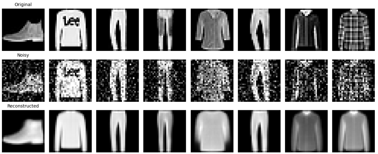

# ============================================================================
# VISUALIZATION : NOISE ROBUSTNESS TEST
# Tests model performance at different noise levels (0.1 to 0.6)
# Shows how well the model handles varying amounts of noise
# ============================================================================
import random

img_idx = random.randint(0, images.size(0) - 1)
noise_levels = [0.1, 0.25, 0.4, 0.6]

plt.figure(figsize=(12, 8))

for i, nf in enumerate(noise_levels):
    noisy_test = add_noise(images, nf)
    with torch.no_grad():
        recon, _ = model(noisy_test)
        
    # Original
    plt.subplot(len(noise_levels), 3, i*3 + 1)
    plt.imshow(images[img_idx].cpu().squeeze(), cmap='gray')
    plt.axis('off')
    if i == 0:
        plt.title('Original', fontsize=10)
    plt.ylabel(f'Noise={nf}', fontsize=9)
    
    # Noisy
    plt.subplot(len(noise_levels), 3, i*3 + 2)
    plt.imshow(noisy_test[img_idx].cpu().squeeze(), cmap='gray')
    plt.axis('off')
    if i == 0:
        plt.title('Noisy Input', fontsize=10)
        
    # Reconstructed
    plt.subplot(len(noise_levels), 3, i*3 + 3)
    plt.imshow(recon[img_idx].view(28,28).cpu(), cmap='gray')
    plt.axis('off')
    if i == 0:
        plt.title('Reconstructed', fontsize=10)

plt.suptitle('Denoising Performance at Different Noise Levels', fontsize=12)
plt.tight_layout()
plt.savefig('noise_comparison.png', dpi=150, bbox_inches='tight')
plt.show()

print("Noise robustness test completed!")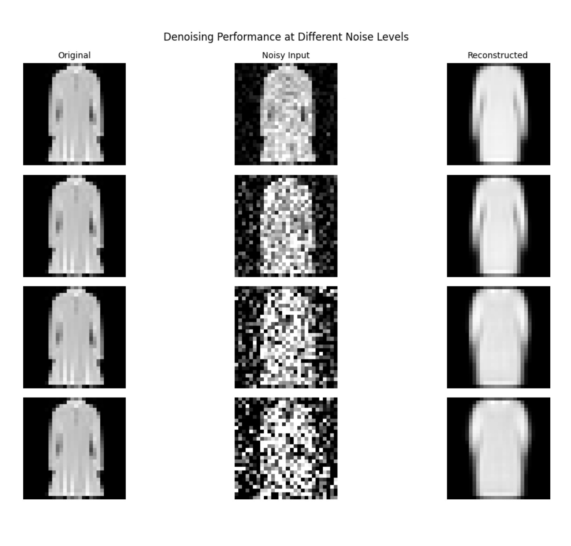

def get_latents(mdl, loader):
    latents, labels = [], []
    with torch.no_grad():
        for images, lbls in loader:
            images = images.to(device)
            _, z = mdl(images)
            latents.append(z.cpu())
            labels.append(lbls)
    return torch.cat(latents).numpy(), torch.cat(labels).numpy()

class_names = [
    "T-shirt/top", "Trouser", "Pullover", "Dress", "Coat",
    "Sandal", "Shirt", "Sneaker", "Bag", "Ankle boot"
]

basic_latents, labels = get_latents(basic_model, test_loader)
denoise_latents, _ = get_latents(model, test_loader)

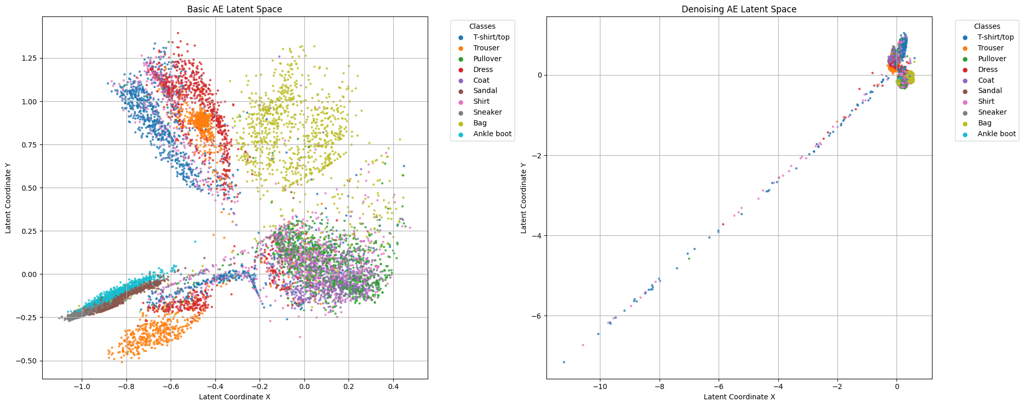
fig, axes = plt.subplots(1, 2, figsize=(20, 8))

for ax, latents, title in zip(axes, 
                               [basic_latents, denoise_latents], 
                               ["Basic AE Latent Space", "Denoising AE Latent Space"]):
    scatter = ax.scatter(latents[:, 0], latents[:, 1], c=labels, cmap='tab10', s=5, alpha=0.7)
    handles = [ax.scatter([], [], c=[scatter.cmap(scatter.norm(i))], label=class_names[i], s=30)
               for i in range(len(class_names))]
    ax.legend(handles=handles, title="Classes", bbox_to_anchor=(1.05, 1), loc='upper left')
    ax.set_xlabel("Latent Coordinate X")
    ax.set_ylabel("Latent Coordinate Y")
    ax.set_title(title)
    ax.grid(True)

plt.tight_layout()
plt.show()

print("Latent space visualization completed!")

def calculate_ssim(img1, img2):
    C1, C2 = 0.01 ** 2, 0.03 ** 2
    mu1, mu2 = img1.mean(), img2.mean()
    sigma1_sq = ((img1 - mu1) ** 2).mean()
    sigma2_sq = ((img2 - mu2) ** 2).mean()
    sigma12 = ((img1 - mu1) * (img2 - mu2)).mean()
    return (((2 * mu1 * mu2 + C1) * (2 * sigma12 + C2)) /
           ((mu1 ** 2 + mu2 ** 2 + C1) * (sigma1_sq + sigma2_sq + C2))).item()

def evaluate_model(mdl, loader, use_noise=False):
    mdl.eval()
    total_mse = total_ssim = total_psnr = total_samples = 0

    with torch.no_grad():
        for images, _ in loader:
            images = images.to(device)
            inputs = add_noise(images) if use_noise else images
            outputs, _ = mdl(inputs)
            outputs = outputs.view_as(images)

            for i in range(images.size(0)):
                mse = ((outputs[i] - images[i]) ** 2).mean().item()
                total_mse += mse
                # Safe PSNR: clamp MSE to avoid log(0)
                total_psnr += 20 * np.log10(1.0 / np.sqrt(max(mse, 1e-10)))
                total_ssim += calculate_ssim(images[i].squeeze(), outputs[i].squeeze())
                total_samples += 1

    return {
        "MSE": total_mse / total_samples,
        "PSNR": total_psnr / total_samples,
        "SSIM": total_ssim / total_samples
    }

# Evaluate both models
basic_metrics = evaluate_model(basic_model, test_loader, use_noise=False)
denoise_metrics = evaluate_model(model, test_loader, use_noise=True)

print("Quantitative Evaluation Results:")
print(f"{'Metric':<10} {'Basic AE':>12} {'Denoising AE':>14}")
print("-" * 38)
for metric in ["MSE", "PSNR", "SSIM"]:
    unit = " dB" if metric == "PSNR" else ""
    print(f"{metric:<10} {basic_metrics[metric]:>11.4f}{unit}  {denoise_metrics[metric]:>11.4f}{unit}")